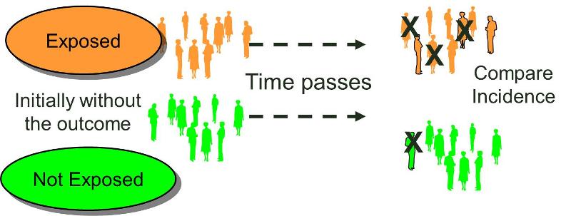
The characteristic feature of a cohort study is that the investigator identifies subjects at a point in time when they do not have the outcome of interest and compares the incidence of the outcome of interest among groups of exposed and unexposed (or less exposed) subjects. (We can refer to the groups being compared as exposure cohorts.) Cohorts may be identified retrospectively or prospectively, but in either case the outcome status needs to be established at least twice. It must be established that a cohort did not have the outcome of interest at the beginning of the observation period, and the cohort needs to be examined again to determine whether or not the outcome subsequently developed, i.e., the incidence in each of the exposure groups.
Upon successful completion of this section of the course, the student will be able to:
- Prospective cohort study
- Retrospective cohort study
- An internal comparison group
- An external comparison group
- A general population comparison group
There are two fundamental types of cohort studies based on when and how the subjects are enrolled into the study:
In prospective cohort studies the investigators conceive and design the study, recruit subjects, and collect baseline exposure data on all subjects, before any of the subjects have developed any of the outcomes of interest. The subjects are then followed into the future in order to record the development of any of the outcomes of interest. The follow up can be conducted by mail questionnaires, by phone interviews, via the Internet, or in person with interviews, physical examinations, and laboratory or imaging tests. Combinations of these methods can also be used.
Typically, the investigators have a primary focus, for example, to learn more about cardiovascular disease or cancer, but the data collected from the cohort over time can be used to answer many questions and test many possible determinants, even factors that they hadn't considered when the study was originally conceived.
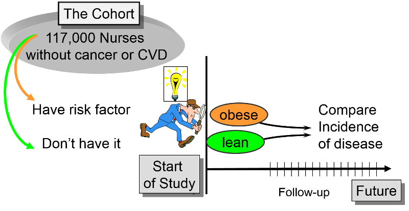
The Framingham Heart Study, the Nurses Health Study, and the Black Women's Health Study are good examples of large, productive prospective cohort studies. In each of these studies, the investigators wanted to study risk factors for common chronic diseases. The investigators identified a cohort (group) of possible subjects who would be feasible to follow for a prolonged period. Eligible subjects had to meet certain criteria (inclusion criteria) to be included in the study as subjects. The investigators then determine the initial or "baseline" characteristics, behaviors, and other "exposures" of all subjects at the beginning of the study. Information is collected from all subjects in the same way using exactly the same questions and data collection methods for all subjects. They design the questions and data collection procedures very carefully in order to have accurate information about exposures before disease develops in any of the subjects.
For more information:
Link to Framingham Heart Study
Link to The Nurses Health Study
Link to The Black Women's Health Study
Of course, data analysis cannot take place until enough 'events' or 'outcomes' have occurred, so time must elapse, and the analyses will look at events that have occurred during the period of time from the beginning of the study until the time of the analysis or the end of the study. It goes without saying that analysis is always done retrospectively, because a span of time has to have elapsed before you can compare incidence. The thing that makes prospective cohort studies prospective is that they were designed prospectively, and subjects were enrolled and had baseline data collected before any of them developed any of the outcomes of interest. Determining baseline exposure status before disease events occur gives prospective studies an important advantage in reducing certain types of bias that can occur in retrospective cohort studies and case-control studies, though at the cost of efficiency.
After baseline information is collected, subjects in a prospective cohort study are then followed "longitudinally," i.e. over a period of time, usually for years. This enables the investigators to know when follow up began, if and when subjects become diseased, if and when they become lost to follow up, and whether their exposure status changed during the follow up period. By having individual data on these details for each subject, the investigators can compute and compare the incidence rates for each of the exposure groups.
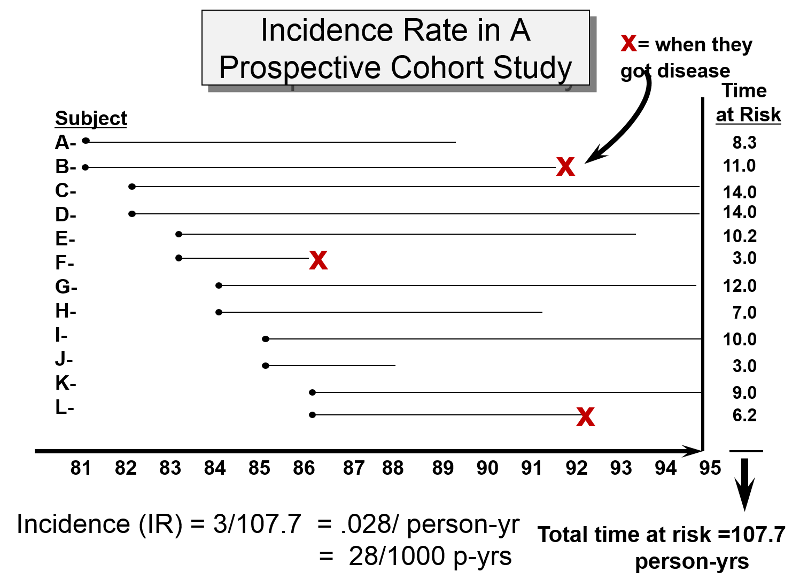
The illustration below shows a hypothetical group of 12 subjects followed over a number of years. They were enrolled into the study at different times, and some of them became lost to follow up, i.e., they stopped responding to letters, emails and phone calls, so we don't know what happened to them; these are show by the horizontal follow up line stopping.
 became lost to follow up." width="500" height="366" />
Three subjects developed the outcome of interest at the approximate dates show by the "X"s. The incidence rate was calculated by computing the disease free observation time for each subject, adding up the disease-free observation times for the entire group, and then dividing this into the number of events, as shown in the calculation below the time line.
Since the investigators asked about many exposures during baseline data collection, they can eventually use the data to study many associations between different exposures and disease outcomes. For example, one could identify smokers and non-smokers at baseline and compare their subsequent incidence of developing heart disease. Alternatively, one could group subjects based on their body mass index (BMI) and compare their risk of developing heart disease or cancer.
The data in the table below summarizes some of the results in a study is from the Nurses' Health Study in which they examined the association of body mass index (BMI) with heart disease. (Link to the article)
Body Mass Index
# Non-fatal Heart Attacks
Person-Years of Observation
MI Rate per 100,000 Person-Years
There were over 118,000 nurses in the study, and they divided the cohort int0 five exposure groups based on BMI. In this case they used the incidence rate of myocardial infarctions (MI, i.e., heart attacks) in the leanest women (BMI < 21) as a reference, against which they compared the incidence rates of MI in the other four groups. For example, the incidence rate of MI in the reference group (those with BMI < 21) was 23.1 per 100,000 person-years of disease-free observation time. The incidence rate in the heaviest group (BMI >29) was 85.4 MIs per 100,000 person-years.
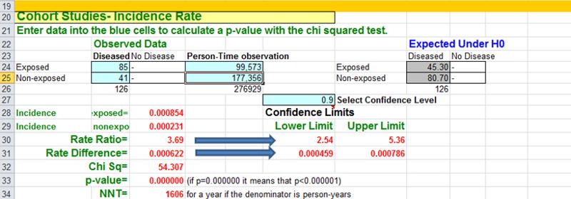
The Epi-Tools.XLS worksheet for cohort studies can compare either cumulative incidence (top section of the worksheet) or incidence rates like these (lower section of the worksheet). For example, if one were to compare the heaviest group (BMI > 29) to the women with BMI < 21 (the reference group), the Epi-Tools analysis would look like this
Manson et al. also used the Nurses' Health Study (NHS) to examine the effect of exercise on cardiovascular disease. The NHS enrolled 121,700 female RNs in 1976, but they didn't begin to collect information on exercise until 1986. Since the original baseline data did not include information on exercise, the exercise study only used the women who had not yet developed any cardiovascular problems by 1986. So, the exercise study was restricted to the 72,448 subjects who were free of cardiovascular disease and cancer in 1986. In essence, the information on exercise and activity that they began collecting in 1986 represented a new baseline for this subset of the original cohort.
Link to the article by Manson et al.
Retrospective studies also group subjects based on their exposure status and compare their incidence of disease. However, in this case both exposure status and outcome are ascertained retrospectively.
In essence, the investigators jump back in time to identify a useful cohort which was initially free of disease and 'at risk.' They then use whatever records are available to determine each subject's exposure status at the begin of the observation period, and they then ascertain what subsequently happened to the subjects in the two (or more) exposure groups. Retrospective cohort studies are also 'longitudinal,' because they examine health outcomes over a span of time. The distinction is that in retrospective cohort studies all of the cases of disease have already occurred before the investigators initiate the study. In contrast, exposure information is collected at the beginning of prospective cohort studies before any subjects have developed any of the outcomes or interest, and the 'at risk' period begins after baseline exposure data is collected and extends into the future.
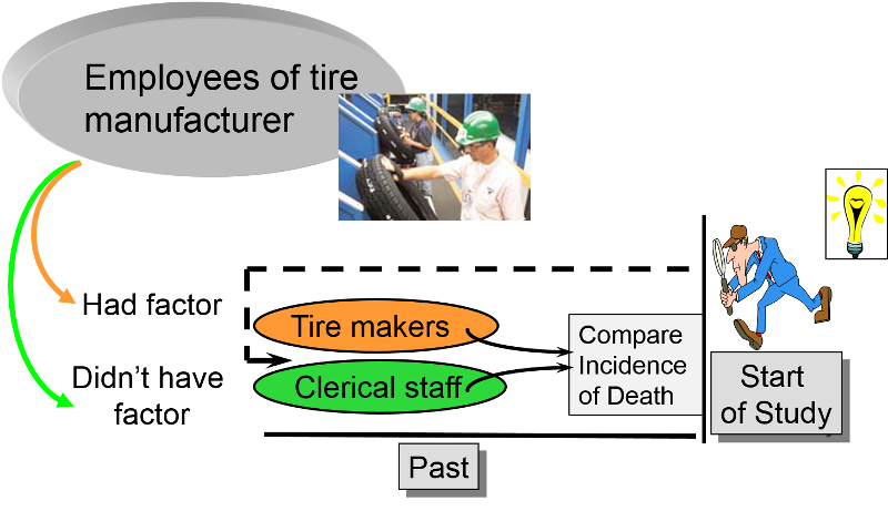
Retrospective cohort studies are particularly useful for unusual exposures or occupational exposures. For example, if an investigator wanted to determine whether exposure to chemicals used in tire manufacturing was associated with an increased risk of death, one might find a tire manufacturing factory that had been in operation for several decades. One could potentially use employee health records to identify those who had had jobs which involved exposure to the chemicals in question (e.g., workers who actually manufactured tires) and non-exposed coworkers (e.g., clerical workers or sales personnel in the same company or, even better, workers also involved in manufacturing operations but with jobs that didn't involve exposure to the chemicals). One could then ascertain what had happened to all the subjects and compare the incidence of death in the exposed and non-exposed workers.
Retrospective cohort studies like this are very efficient because they take much less time and cost much less than prospective cohort studies, but this advantage also creates potential problems. Sometimes exposure status is not clear when it is necessary to go back in time and use whatever data was available, because the data being used was not designed to be used in a study. Even if it was clear who was exposed to tire manufacturing chemicals based on employee records, it would also be important to take into account (or adjust for) other differences that could have influenced mortality (confounding factors). For example, in a study comparing mortality rates between workers exposed to solvents used in tire manufacture and an unexposed comparison group, it might be important to adjust for confounding factors such as smoking and alcohol consumption. However, it is unlikely that a retrospective cohort study would have accurate information on these other risk factors.
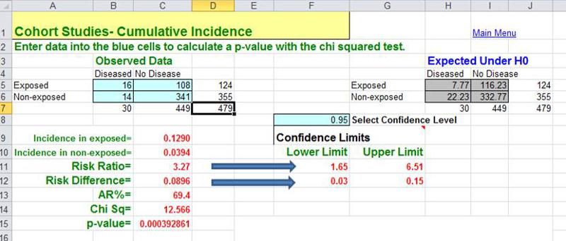
When an outbreak of Giardia (see this Link to CDC page on Giardia) occurred in Milton, MA , the Milton Health Department requested assistance from the epidemiologists in the MA Department of Public Health. (Kathleen MacVarish from the BUSPH Practice Office was the Health Agent in Milton who led the investigation.) The request for assistance was made some time after the start of the outbreak, and the outbreak was winding down by the time DPH began their study. The outbreak was clearly concentrated among members of the Wollaston Golf Club in Milton, MA , which had two swimming pools, one for adults and a wading pool for infants and small children. Given what they knew about the usual mechanisms by which Giardia is transmitted, the investigators thought that contamination of the kiddy pool by a child shedding Giardia into their stool was the most likely source. (NOTE) The study was conducted by getting most of the people in the cohort to complete a questionnaire in which one of the key questions was "Did you spend any time in the kiddy pool?" This outbreak clearly took place in a well-defined cohort (members of the club), and the investigators could determine how many people developed Giardia in each of the exposure groups (i.e., exposed to the kiddy pool or not). Moreover, they also knew how many respondents had been exposed to the kiddy pool and how many were not. In other words, they knew the denominators for the exposure groups, so they could calculate the cumulative incidence, risk difference, and the risk ratio. They found that people who had spent time in the kiddy pool had 9.0 more cases per 100 persons than those who spent time in the kiddy pool. The risk ratio was 3.27. Because the investigation started after the cases had already occurred, DPH's study of Giardia in Milton is an example of a retrospective cohort study.
A cohort study may also be ambidirectional , meaning that there are both retrospective and prospective phases of the study. Ambidirectional studies are much less common than purely prospective or retrospective studies, but they are conceptually consistent with and share elements of the advantages and disadvantages of both types of studies. The Air Force Health Study (AFHS) - also known as the Ranch Hand Study - was initiated by the U. S. Air Force in 1979 to assess the possible health effects of military personnel's exposure to Agent Orange and other chemical defoliants sprayed during the Vietnam War. The study was conducted comparing:
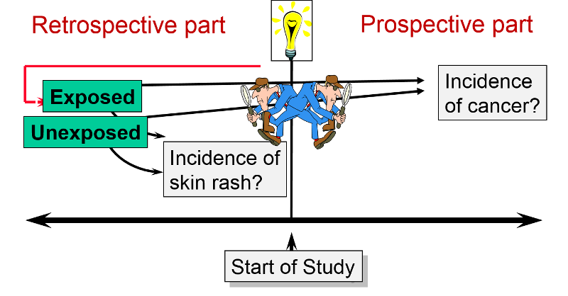
This is an "ambidirectional" study, because it had both a retrospective component and a prospective component. Some of the problems suspected to be caused by Agent Orange would have occurred shortly after exposure (e.g., skin rashes). These were addressed by looking at the cohort retrospectively to see if the exposed pilots had had more problems than the controls. Other problems (e.g., infertility & cancer) might not surface until some time after the exposure. Therefore, the cohort was followed prospectively to see if they had a greater incidence of these problems. The reports that emerged from the study suggested links between Agent Orange exposure and nine distinct diseases: chloracne, Hodgkin's disease, multiple myeloma, non- Hodgkin's lymphoma, porphyria cutanea tarda, respiratory cancers (lung, bronchus, larynx and trachea), soft-tissue sarcoma, acute and subacute peripheral neuropathy, and prostate cancer.
A closed cohort is one with fixed membership. Once the cohort is defined by enrolling subjects and follow up begins, no one can be added. The number of subjects may decline because of death or loss to follow up, but no additional subjects are added. As a result, closed cohorts always get smaller over time. Citizens of Japan who were exposed to radiation when atomic bombs were dropped on Hiroshima and Nagasaki during the second World War, would be considered members of a fixed or closed cohort that was defined by an event. Ashengrau and Seage would classify the bombing victims as a "fixed cohort" and make a distinction between a fixed cohort and a closed cohort. They define a closed cohort as similar to a fixed cohort except that a closed cohort is one that has no losses to follow up, for example, a cohort of people who attended a luncheon that resulted in an outbreak of Salmonellosis.
In contrast, an open cohort is dynamic, meaning that members can leave or be added over time. Rothman gives the example of a state cancer registry. Subjects are continually added when they are diagnosed with cancer, so new subjects are continually added. Subjects can also leave the cohort by moving to a new state or dying. Another example of an open or dynamic cohort would be students at Boston University.
These descriptions should sound familiar, because they essentially parallel the descriptions of fixed and dynamic populations from the Measures of Disease Frequency module. The great majority of cohort studies are conducted in closed (or fixed) cohorts, because it is more difficult to establish eligibility and track people in an open cohort, since they can enter and leave at any time. This problem becomes greater as the size of the cohort gets larger and/or the study continues for a longer period of time. Note that the retrospective cohort study of Giardia in Milton was an open cohort (members of the golf club), but the population was relatively small and time period very short.
For common risk factors, (e.g., smoking, obesity) investigators may enroll a general population cohort, e.g.,
Once a general population cohort is enrolled, investigators will ascertain their baseline exposures to a large number of exposures of interest and possible confounding factors that they may need to adjust for in the analyses.
For uncommon risks, investigators use special exposure cohorts, e.g.,
The ideal comparison group in a cohort study would be a group that was exactly the same as the exposed group, except that they would be unexposed. This is referred to as the "counterfactual ideal," because it is impossible for the same person to be both exposed and unexposed at the same time. Consequently, the best one can do is to select a comparison group that differs with respect to the exposure of interest but is a similar as possible with respect to other factors that might influence the outcome. There are two key things that are essential in selecting the comparison group in a cohort study:
There are three general types of comparison groups for cohort studies.
Internal Comparison Group
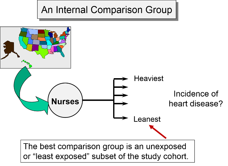
An internal comparison group consists of unexposed members of the same cohort. This is generally the best comparison group, because the subjects are comparable in many respects. For example, as noted earlier, the Nurses' Health Study, used the cohort to study a possible association between obesity and myocardial infarction. Subjects from the cohort were categorized into one of five levels of body mass index, and the group with the lowest BMI was used as an internal comparison group or reference group, against which the other categories were compared.
External Comparison Group
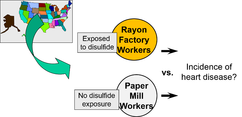
When it isn't possible to take a well-defined cohort and divide it into exposure groups, sometimes one can identify an external comparison cohort. This type of comparison group was used when researchers wanted to look at occupational exposure to disulfide in rayon factory workers. Because virtually all workers in the plant were exposed to disulfide, it was not possible to use an internal comparison group from the same plant. Instead, they selected a group of people employed in a paper mill as an external comparison cohort. Both groups had similar education, age, socioeconomic status, and gender distribution. However, they may have differed with respect to other important confounding factors.
General Population as a Comparison Group
The third possibility is to use the general population as a comparison group. This is used occasionally in situations where only a small percentage of the population is exposed, e.g., with an unusual occupational exposure. However, the general population may differ from the exposed work force in many ways, including overal health.
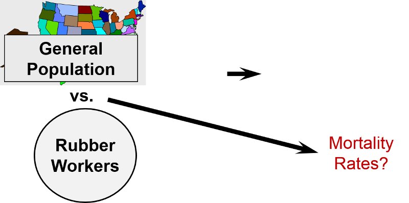
One study looked at mortality rates of workers in the rubber industry and compared them to the general population of the US. There are several problems with this. 1) Some of the general population will have had the exposure (same occupation); 2) the general population includes people who are unable to work because of illness or disability. Employed workers tend to be healthier than the general population. This is a well-documented phenomenon know as the "healthy worker effect." Rates of disease and death tend to be higher in the general population than in the employed work force because the general population includes many people who are too sick or disabled to work. As a result, even if the exposure was, in fact, associated with higher mortality, the magnitude of association would be underestimated because of the inherently higher mortality rate in the general population (which includes both employed and unemployed workers). Although this is not a problem with all diseases, the general population generally exhibits the greatest departure from the counterfactual ideal, and therefore is less widely used today than in the past. Another notable disadvantage of the general population comparison group is that data on important confounders are almost never available.
The use of the general population as a comparison group is most likely to be seen today in descriptive epidemiology, particularly when there are many categories of exposure with only a small number of outcomes per category. For example, the Massachusetts Cancer Registry reports the cancer rate in each of 351 cities and towns using the overall rate in the general population as a comparison. Similarly, descriptions of occupational mortality based on death certificate data may have hundreds of different occupations and also use the general population as a comparison group.
Studies of this type sometimes use a standardized mortality ratio (SMR) as the measure of association. Data from the general population provide overall rates of mortality in the population. These rates are then used to predict how many deaths would be expected in the cohort under study. The SMR is the ratio of observed deaths in the cohort to the number of deaths expected. The SMR is interpreted much like a risk ratio. For example, an SMR=1.2 indicates 1.2 times the risk in the general population or a 20% increase in risk. (Note that sometimes the SMR is multiplied x 100; if so, SMR=120 would also indicate a 20% increase in risk. If population rates are available by age, gender, and race, then SMRs can be adjusted or "standardized" to control for confounding by these factors. This is a method sometimes referred to as "indirect standardization."
A similar analytical approach is used to compute standardized incidence ratios (SIR). For example, the Massachusetts Cancer Registry uses the general population of Massachusetts as a comparison group in order to examine whether the incidence of specific cancers differs in individual communities compared to the entire state's incidence. In this setting the measure of association that is used is a standardized incidence ratio (SIR). SIRs can also be interpreted much like a risk ratio, although they are typically multiplied by 100, so that SIR=120 would indicate an incidence that was 20% greater than that in the overall population.
Link to the Massachusetts Cancer Registry
Link to BUSPH learning module on Standardized Rates and page on Standardized Incidence Ratios
Selection bias from enrollment procedures rarely occurs in cohort studies, because the outcomes have not yet occurred at the time when subjects are enrolled, so a potential participant's eventual outcome status is unknown and therefore can not influence . However, selection bias can occur in a prospective cohort study as a result of differences in retention during the follow-up period after enrollment. When the observation period spans many years (in either retrospective or prospective cohort studies) it can be difficult to track subjects for the entire study. Subjects may disappear as a result of death, relocation, or (in prospective studies) loss of interest in the study. Studies with follow up rates of less than 60% will generally be seen as having limited validity, but even losses of 20% can introduce bias if the reasons for loss are related to both exposure status and outcome status.
Losses to follow-up can introduce bias (a deviation of the observed value of the measure of association from the value that would have been observed in the absence of bias) if there are differences in likelihood of loss to follow-up that are related to exposure status and outcome. In general, large prospective cohort studies are doing well if they can maintain follow-up of 80-90% of their sample for long periods.
As an illustration of how bias can be introduced with loss to follow-up, consider the following example. Suppose investigators were prospectively studying the association between use of oral contraceptives and development of thromboembolism (TE), i.e., blood clots in veins of the lower extremities or pelvis that can break loose and become lodged in the branches of the pulmonary artery]. Suppose, 20/10,000 OC users developed thromboembolism, but only 10/10,000 controls did, i.e., OC users really had a 2-fold greater risk. If roughly 4,000 subjects were lost to follow-up in each group, and if 12 of the 20 subjects who developed thromboembolism in the OC group became lost to follow-up, but only 2 subjects with thromboembolism were lost in the control group, the differential loss to follow-up would make it appear that rates of thromboembolism were similar, and the estimate of association (risk ratio) would be biased.The bias that can result from this differential follow up is a type of selection bias.
The enrollment of subjects in a prospective cohort study like this would not introduce selection bias, because the outcome has not yet occurred. However, retention of subjects may be differentially related to exposure and outcome, and this has a similar effect that can bias the results. In the hypothetical cohort study below investigators compared the incidence of thromboembolism (TE) in 10,000 women on oral contraceptives (OC) and 10,000 women not taking OC. TE occurred in 20 subjects taking OC and in 10 subjects not taking OC, so the true risk ratio was (20/10,000) / (10/10,000) = 2.